
High-quality calibrated uncertainty estimates are crucial for numerous real-world applications, especially for deep learning-based deployed ML systems. While Bayesian deep learning techniques allow uncertainty estimation, training them with large-scale datasets is an expensive process that does not always yield models competitive with non-Bayesian counterparts. Moreover, many of the high-performing deep learning models that are already trained and deployed are non-Bayesian in nature and do not provide uncertainty estimates. To address these issues, we propose BayesCap that learns a Bayesian identity mapping for the frozen model, allowing uncertainty estimation. BayesCap is a memory-efficient method that can be trained on a small fraction of the original dataset, enhancing pretrained non-Bayesian computer vision models by providing calibrated uncertainty estimates for the predictions without (i) hampering the performance of the model and (ii) the need for expensive retraining the model from scratch. The proposed method is agnostic to various architectures and tasks. We show the efficacy of our method on a wide variety of tasks with a diverse set of architectures, including image super-resolution, deblurring, inpainting, and crucial application such as medical image translation. Moreover, we apply the derived uncertainty estimates to detect out-of-distribution samples in critical scenarios like depth estimation in autonomous driving.
Introduction
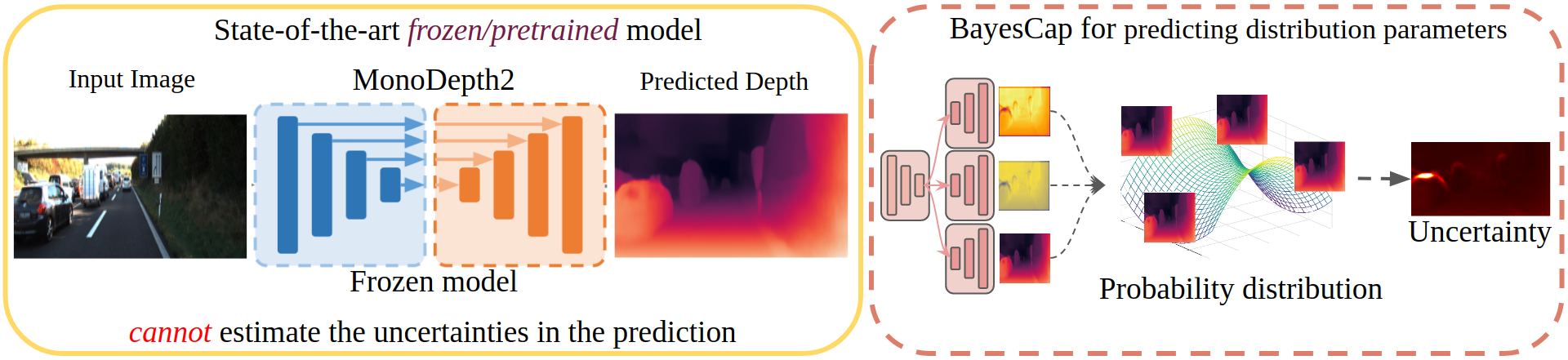 Image enhancement tasks like super-resolution, deblurring, inpainting, colorization, denoising, medical image synthesis and monocular depth estimation among others have been effectively tackled using deep learning methods generating high-fidelity outputs. But, the respective state-of-the-art models usually learn a deterministic one-to-one mapping between the input and the output, without modeling the uncertainty in the prediction. While there have been works that try to learn a probabilistic mapping instead, they are often difficult to train and more expensive compared to their deterministic counterparts. In this work, we propose BayesCap, an architecture agnostic, plug-and-play method to generate uncertainty estimates for pre-trained models. The key idea is to train a Bayesian autoencoder over the output images of the pretrained network, approximating the underlying output distribution. Due to its Bayesian design, in addition to reconstructing the input, BayesCap also estimates the parameters of the underlying distribution, allowing us to compute the uncertainties. BayesCap is highly data-efficient and can be trained on a small fraction of the original dataset.
Problem Formulation
Let be the training set with pairs from domain and (i.e., ), where lies in and , respectively. While our proposed solution is valid for data of arbitrary dimension, we present the formulation for images with applications for image enhancement and translation tasks, such as super-resolution, inpainting, etc. Therefore, () represents a pair of images, where refers to the input and denotes the transformed / enhanced output. For instance, in super-resolution is a low-resolution image and its high-resolution version. Let represent a Deep Neural Network parametrized by that maps images from the set to the set , e.g. from corrupted to the non-corrupted / enhanced output images.
We consider a real-world scenario, where has already been trained using the dataset and it is in a frozen state with parameters set to the learned optimal parameters . In this state, given an input , the model returns a point estimate of the output, i.e., . However, point estimates do not capture the distributions of the output () and thus the uncertainty in the prediction that is crucial in many real-world applications. Therefore, we propose to estimate for the pretrained model in a fast and cheap manner, quantifying the uncertainties of the output without re-training the model itself.
Preliminaries: Uncertainty Estimation
 To understand the functioning of our BayesCap that produces uncertainty estimates for the frozen or pretrained neural networks, we first consider a model trained from scratch to address the target task and estimate uncertainty. Let us denote this model by , with a set of trainable parameters given by . To capture the irreducible (i.e., aleatoric) uncertainty in the output distribution , the model must estimate the parameters of the distribution. These are then used to maximize the likelihood function. That is, for an input , the model produces a set of parameters representing the output given by, , that characterizes the distribution , such that . The likelihood is then maximized in order to estimate the optimal parameters of the network. Moreover, the distribution is often chosen such that uncertainty can be estimated using a closed form solution depending on the estimated parameters of the neural network, i.e.,
It is common to use a heteroscedastic Gaussian distribution for , in which case is designed to predict the mean and variance of the Gaussian distribution, i.e., , and the predicted variance itself can be treated as uncertainty in the prediction. The optimization problem becomes,
The above equation models the per-pixel residual (between the prediction and the ground-truth) as a Gaussian distribution. However, this may not always be fit, especially in the presence of outliers and artefacts, where the residuals often follow heavy-tailed distributions. Recent works such as have shown that heavy-tailed distributions can be modeled as a heteroscedastic generalized Gaussian distribution, in which case is designed to predict the \textit{mean} (), \textit{scale} (), and \textit{shape} () as trainable parameters, i.e., ,
Here , represents the Gamma function. While the above formulation shows the dependence of various predicted distribution parameters on one another when maximizing the likelihood, it requires training the model from scratch, that we want to avoid. In the following, we describe how we address this problem through our BayesCap.
Constructing BayesCap
In the above, was trained from scratch to predict all the parameters of distribution and does not leverage the frozen model estimating using in a deterministic fashion. To circumvent the training from scratch, we notice that one only needs to estimate the remaining parameters of the underlying distribution. Therefore, to augment the frozen point estimation model, we learn a Bayesian identity mapping represented by , that reconstructs the output of the frozen model and also produces the parameters of the distribution modeling the reconstructed output. We refer to this network as BayesCap. We use heteroscedastic generalized Gaussian to model output distribution, i.e.,
To enforce the identity mapping, for every input , we regress the reconstructed output of the BayesCap () with the output of the pretrained base network (). This ensures that, the distribution predicted by BayesCap for an input , i.e., , is such that the point estimates match the point estimates of the pretrained network . Therefore, as the quality of the reconstructed output improves, the uncertainty estimated by also approximates the uncertainty for the prediction made by the pretrained , i.e.,
To train and obtain optimal parameters (), we minimize the fidelity term between and , along with the negative log-likelihood for , i.e.,
Here represents the hyperparameter controlling the contribution of the fidelity term in the overall loss function. Extremely high will lead to improper estimation of the () and () parameters as other terms are ignored. Above equation allows BayesCap to estimate the underlying distribution and uncertainty.
Results
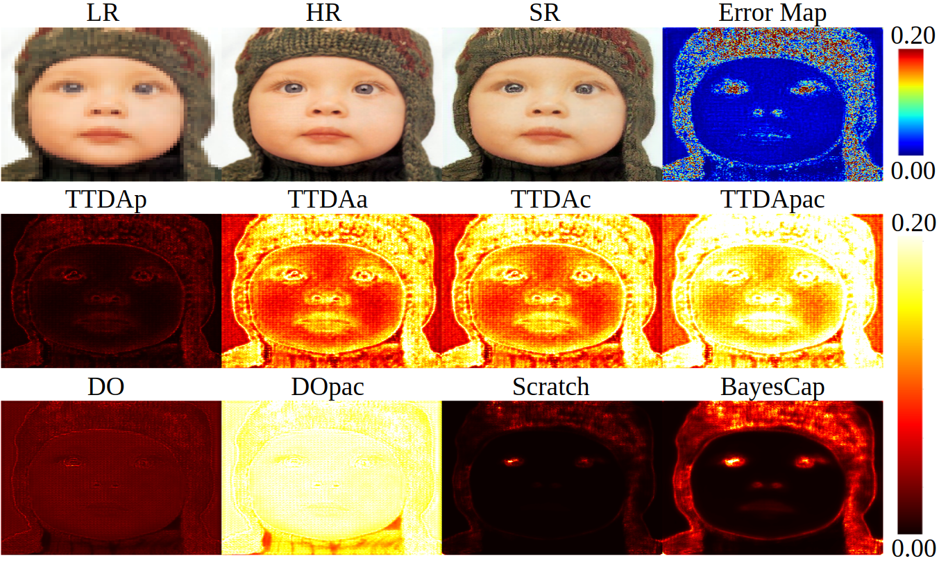
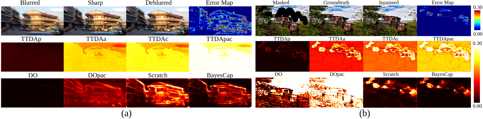
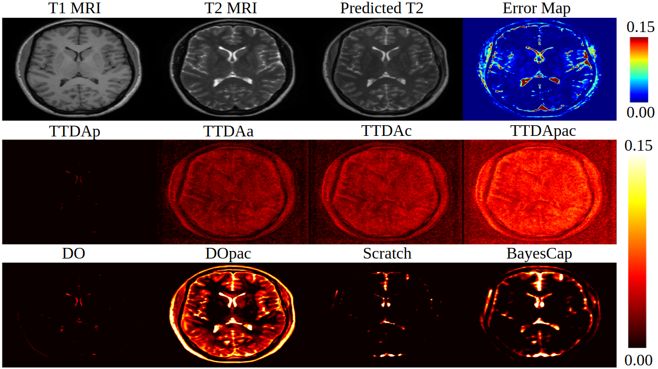
We test our method BayesCap on the tasks of image super-resolution, deblurring, inpatining and medical image translation. In all the tasks, we are able to retain the outputs of the base model while also providing uncertainty estimates. For all tasks, we compare BayesCap against 7 methods in total, out of which 6 baselines can estimate uncertainty of a pretrained model without re-training and one baseline modifies the base network and train it from scratch to estimate the uncertainty. The first set of baselines belong to test-time data augmentation (TTDA) technique, where we generate multiple perturbed copies of the input and use the set of corresponding outputs to compute the uncertainty. We consider three different ways of perturbing the input, (i) per-pixel noise perturbations (TTDAp), (ii) affine transformations (TTDAa) and (iii) random corruptions from Gaussian blurring, contrast enhancement, and color jittering (TTDAc). As additional baseline, we also consider TTDApac that generates the multiple copies by combining pixel-level perturbations, affine transformations, and corruptions as described above.
Some results are illustrated below:
Super-Resolution
Deblurring and Inpainting
Medical Image Translation
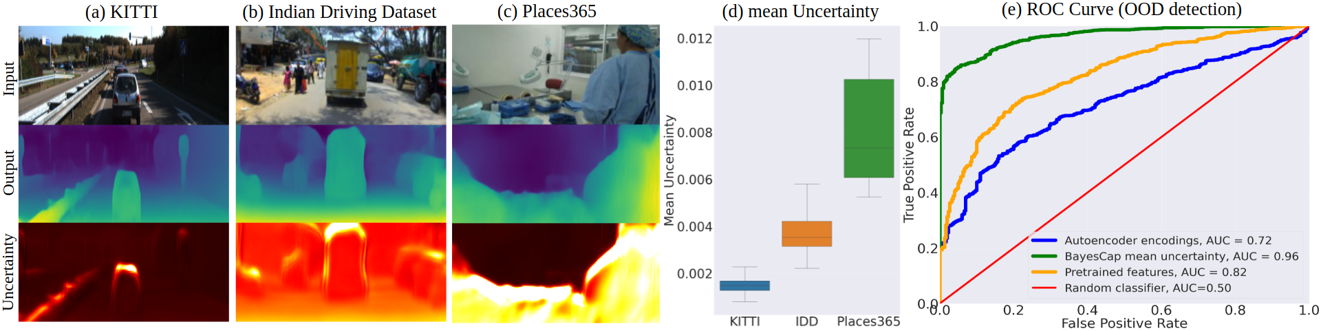
In addition to this, we also show the downstream benefits of uncertainty estimation. In the case of monocular depth estimation for autonomous driving, we show that BayesCap can be used to detect out-of-distribution samples which are captured either from different geographies and scenes.
For more results and analysis, please refer to the paper. You can also find a demo of our work here.