
Recent advances have indicated the strengths of self-supervised pre-training for improving representation learning on downstream tasks. Existing works often utilize self-supervised pre-trained models by fine-tuning on downstream tasks. However, fine-tuning does not generalize to the case when one needs to build a customized model architecture different from the self-supervised model. In this work, we formulate a new knowledge distillation framework to transfer the knowledge from self-supervised pre-trained models to any other student network by a novel approach named Embedding Graph Alignment. Specifically, inspired by the spirit of instance discrimination in self-supervised learning, we model the instance-instance relations by a graph formulation in the feature embedding space and distill the self-supervised teacher knowledge to a student network by aligning the teacher graph and the student graph. Our distillation scheme can be flexibly applied to transfer the self-supervised knowledge to enhance representation learning on various student networks. We demonstrate that our model outperforms multiple representative knowledge distillation methods on three benchmark datasets, including CIFAR100, STL10, and TinyImageNet.
Introduction
Self-supervised learning models are recently shown to be successful unsupervised learners that could greatly boost representation learning on different downstream tasks. By fine-tuning a self-supervised pre-trained model, self-supervised knowledge can often bring more advanced model performance in a wide variety of downstream tasks, such as image classification, object detection, and instance segmentation. However, fine-tuning a self-supervised model could be undesirable in several aspects.
In this work, to leverage the strength of self-supervised pre-trained networks, we explore the knowledge distillation paradigm to transfer knowledge from a self-supervised pre-trained teacher model to a small, lightweight supervised student network. Given that the most representative self-supervised models are often trained to learn discriminative representations through instance-wise supervision signals, we hypothesize that these self-supervised teacher models offer a good structural information among different instances.
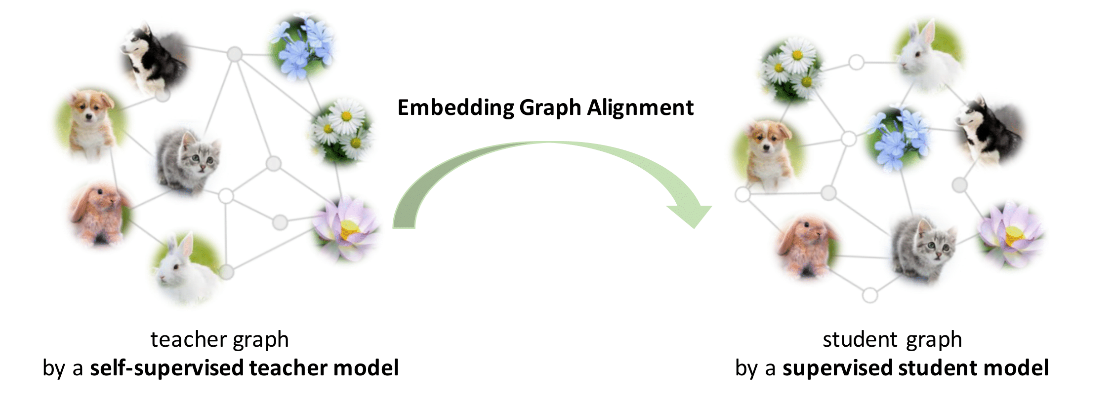
To distill such fine-grained structural information learned by a self-supervised pre-trained model, we propose to model the instance-instance relationships by a graph structure in the embedding space and distill such the structural information among instances by aligning the teacher graph and the student graph.
Model
Overview
Our goal is to distill the knowledge learned from a self-supervised pre-trained teacher model to enhance the visual representation learning of a supervised student model on a visual recognition task.
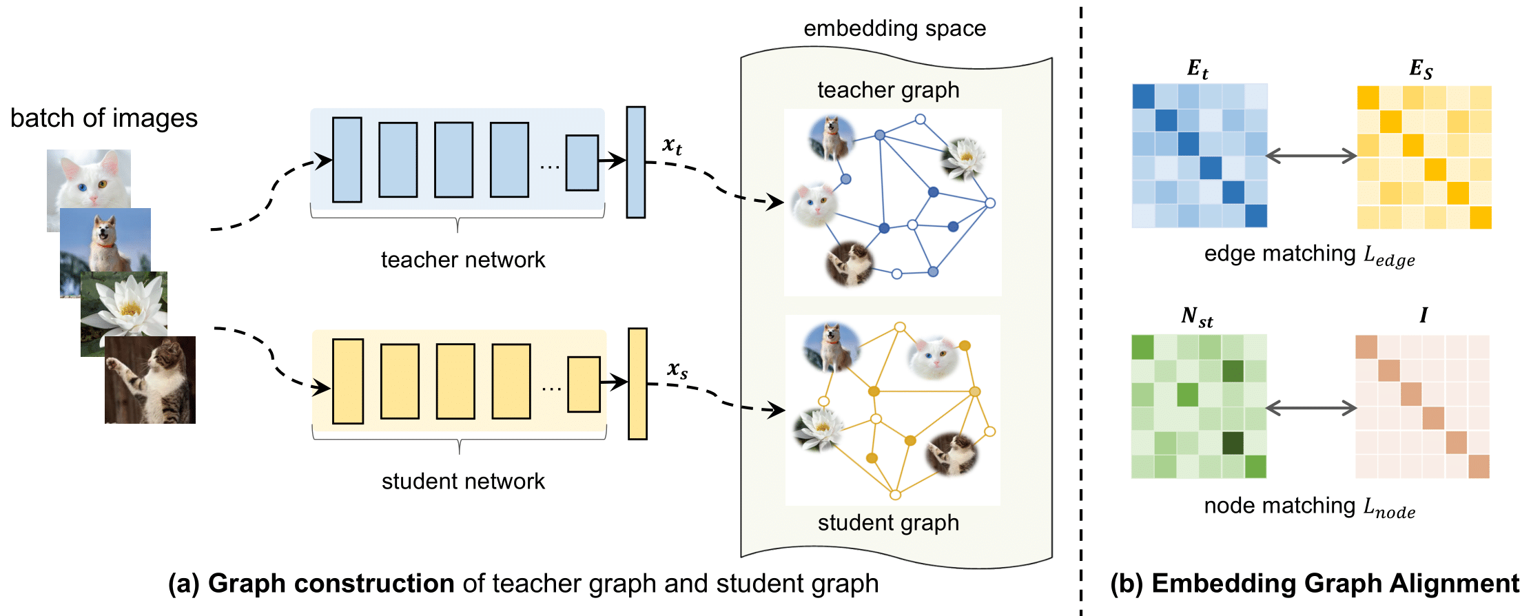 Figure presents the model overview of our proposed Embedding Graph Alignment (EGA) approach for distilling the knowledge from a self-supervised teacher network to a supervised student network. Given a batch of image samples , we first feed the input samples to the teacher network and the student network respectively, resulting in a batch of teacher feature embeddings and a batch of student feature embeddings . To represent the geometry and correlations among different feature embeddings, we construct a graph in the embedding space to encode the instance-instance relationships. For distilling the knowledge, we align the teacher graph and the student graph by jointly optimizing an edge matching constraint and a node matching constraint, which work synergistically to align the features between teacher and student networks, and transfer the instance-instance correlations from the teacher to the student.
Graph Construction
To capture the fine-grained structural information in the embedding space, we construct a graph to encode the structural correlations among a batch of embeddings, where refers to a set of nodes (also known as vertices), and represents a set of edges that encode the structural correlations among different instances: . In the following, we detail how we compute the node embedding and the edge to construct the graph in the embedding space.
Node
To learn the node embedding, we feed the extracted features from the teacher and student networks to individual node embedding layers (which are parameterized as linear projection layers). This also allows the different teacher and student networks to be deployed in our framework without checking which network needs an extra projection layer. Let and denote the feature vectors extracted directly from the teacher and student networks. We pass and to the two node embedding layers to obtain the projected embeddings and , where denotes the dimensionality of the embedding space shared between the teacher and the student models. The embeddings , are utilized as the node representations in the teacher graph and the student graph , which capture the high-level semantic information of each input image. To distill knowledge from the teacher to the student model, an intuitive solution is the align the node embeddings , directly through certain learning constraints, which we will detail in Section \ref{sec:matching}.
Edge
To capture the structural correlations among different instances, we propose to derive each edge in the graph to encode the correlation between every pair of images among the same batch based on the Pearson's correlation coefficient (PPC) -- also known as the Pearson product-moment correlation coefficient (PPMCC). Formally, given pairs of data points denoted as where , the correlation coefficient is defined as:
where is the sample size, are the individual data points, are the mean, and are the standard deviation. We apply the above formula to quantify the correlation between every pair of node embedding, and construct the edge based on this correlation. Specifically, given a pair of node embeddings denoted as and (where and ),
we can compute their connected edge in a graph based on Eq. 1, as defined below.
where is the feature dimension.
is the edge that connects the two node embeddings , , and quantifies their relationship through their correlation. Based on Eq. 2, one can build the teacher graph for a batch of node embeddings by computing the edge between every pairs of node embeddings, while the same procedure can be applied for building the student graph. The constructed graph, therefore, encodes the pairwise correlations among all the instances in the same batch.
Embedding Graph Alignment
We first detail how we construct the edge matrix and node matrix, and describe how we formulate our distillation objectives to match the edges and nodes.
Edge matrix
The edge matrix is formulated based on Eq. 2, which encodes all the pairwise correlations among a batch of node embeddings . Let denote the correlation between the embeddings and computed with Eq. 2. We can formulate an edge matrix as:
where is the batch size. All the diagonal elements on are 1, given that its diagonal represents the self-correlations of each individual embedding. With Eq. 3, we can compute the edge matrices for both the teacher model and the student model using their batch of node embeddings: and . Accordingly, we can write their corresponding edge matrices as and , which encodes all the edges in two graphs.
Edge matching
To distill the structural correlation information captured in the teacher graph, we propose to align the edge matrices of the teacher graph and the student graph. Formally, we define an edge matching loss to match the edge information between two graphs, as written below.
where explicitly enforces the student network to distill the same structural correlations learned by the teacher network by aligning the edge matrices and . Once trained with the above constraint, the student network is expected to obtain similar relative relations among different instances in the embedding space.
Node matrix
To encourage the student to mimic the representations learned by the teacher network, we propose to align their node embeddings of the same input image. Specifically, we define a node matrix where each element captures the correlation between the teacher and the student embeddings. We derive this matrix in a similar manner as our formula in Eq. 4:
Conceptually, the node matrix connects the teacher and student embeddings by building an edge among every pair of teacher and student embeddings to quantify the cross-correlations between the teacher and student models, which differs from the edge matrices that quantify the self-correlations among embeddings from the same network.
Node matching
To ensure the embeddings are aligned across the teacher and student networks, we impose the following node matching loss to ensure that the correlation between the teacher and student embeddings of the same input image is high (i.e. close to 1); while the correlation between different input images is low (i.e. close to 0). For this aim, we enforce the node matrix from Eq. 5 to align with an identity matrix , as defined below.
where the node matrix is encouraged to have its diagonal elements as 1 and the rest as 0, given that the diagonal encodes the correlation between the teacher and student embeddings of the same input image, and should yield high correlation values close to 1.
Embedding Graph Alignment
To align the teacher and the student graphs, we impose the embedding graph alignment loss for distillation, which contains two loss terms: the edge matching loss (Eq. 5) and the node matching loss (Eq. 6), as defined below.
where is a hyperparameter to balance two loss terms.
Model Optimization
Our learning objective includes a standard task objective and an embedding graph alignment loss for knowledge distillation. We consider image classification in this work and the task objective is a standard cross-entropy loss . The overall objective can be written as:
Experimental results
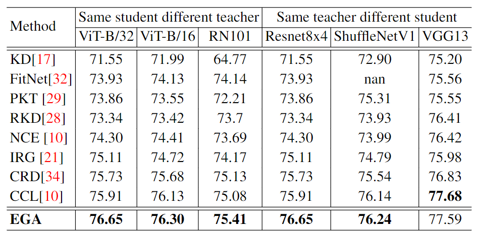
We compare our method to multiple representative state-of-the-art distillation methods.
The results are shown in the following table:
 Besides, we test on CIFAR100, STL-10 and TinyImageNet with different model combinations and different training strategies.
We also analyze the learning dynamics. Figure
Besides, we test on CIFAR100, STL-10 and TinyImageNet with different model combinations and different training strategies.
We also analyze the learning dynamics. Figure
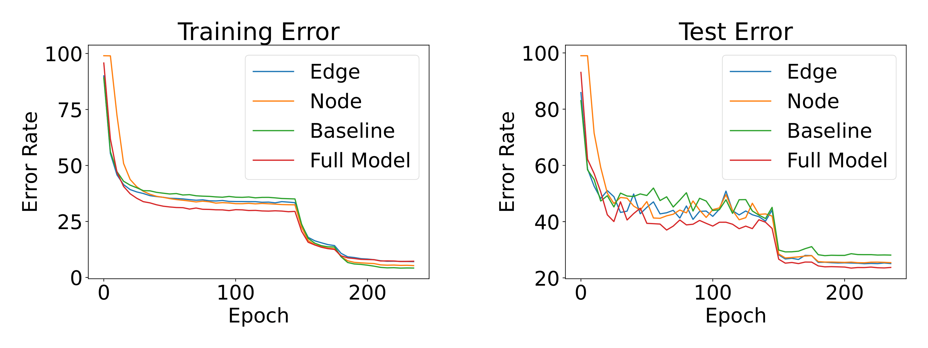
shows the learning curves of different models on CIFAR100. We compare the baseline model (only ), edge matching loss model (), node matching loss model () and our full EGA model. It is interesting to observe that our EGA is less overfitting on the training set compared to other models, especially the baseline. It also proves that our full model formulation EGA performs and generalizes much better than the EGA variants with a single loss term.
In order to examine the distilled structural semantic relationships learned from the teacher network by different loss terms, we visualize the feature embeddings of the EGA. Figure
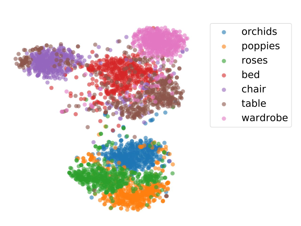 shows that the EGA model can learn the structural semantics and capture the instance-instance relations well.
For more results and analysis, please refer to the paper.