
Compositional Zero-Shot learning (CZSL) aims to recognize unseen compositions of state and object visual primitives seen during training. A problem with standard CZSL is the assumption of knowing which unseen compositions will be available at test time. In this work, we overcome this assumption operating on the open world setting, where no limit is imposed on the compositional space at test time, and the search space contains a large number of unseen compositions. To address this problem, we propose a new approach, Compositional Cosine Graph Embeddings (Co-CGE), based on two principles. First, Co-CGE models the dependency between states, objects and their compositions through a graph convolutional neural network. The graph propagates information from seen to unseen concepts, improving their representations. Second, since not all unseen compositions are equally feasible, and less feasible ones may damage the learned representations, Co-CGE estimates a feasibility score for each unseen composition, using the scores as margins in a cosine similarity-based loss and as weights in the adjacency matrix of the graphs. Experiments show that our approach achieves state-of-the-art performances in standard CZSL while outperforming previous methods in the open world scenario.
Open World Compositional Zero-Shot Learning
Can we recognize state-object compositions (e.g. wet dog, ripe tomato) within ~30k classes? In this blog post, we describe our recent work on compositional zero-shot learning (CZSL) in the open-world scenario, where no constraints exist in the compositional space. We tackle this problem with a method, Co-CGE which assigns a feasibility score to each composition. Co-CGE uses these scores to model the relationship between objects (e.g. dog, tomato), states (e.g. wet, ripe), and their compositions, achieving the new state of the art in CZSL.
What is Compositional Zero-Shot Learning?
Compositional Zero-Shot Learning (CZSL) is the task of recognizing which composition of an object (e.g. dog, tomato) and a state (e.g. wet, ripe) is present in an image. To solve this task, we are given a set of training images containing labels for objects and states of interest, in various compositions. The main challenge of this task is the lack of data. In fact, the training set contains images of a subset of all the compositions of interest (e.g. it may contain wet dog and ripe tomato, but not wet tomato), and we are asked to predict both seen and unseen compositions at test time. This is challenging since the appearance of an object strictly depends on its state (e.g. a wet dog is different from a dry one) and that not all the objects are modified in the same way by the same state (e.g. wet dog vs wet car). This makes it hard to predict the object and the state independently and thus our model must forecast how unseen compositions should look like.
From the Closed to the Open World
Unseen compositions are, by definition, unseen. However, previous works assumed to at least know which unseen compositions will be present at test time. This prior knowledge, allows us to restrict the search space of the model to just seen and the known unseen compositions. As an example, consider one of the most popular CZSL benchmarks, MIT-States. In this benchmark, we have 245 objects and 115 states, for a total of ~28k compositions. Among them, we have 1262 seen compositions, and 400 unseen ones at test time. Thus, we can restrict the search space to the 1662 known test compositions, i.e. ~6% of the full compositional space. Unfortunately, such big restrictions of the search space come with a drawback: excluding from the output space even feasible compositions that our model may find when applied in the real world. As an example, let us suppose we have a set of objects like {cat, dog, tomato} and a set of states like {wet, dry, ripe}. If wet cat is neither among the seen compositions nor in the unknown test ones, it will be automatically excluded from the output space of the model and cannot be predicted (even if wet cats exist and are pretty funny).
We argue that, for building CZSL systems applicable in the real world, we need to remove the assumption of knowing the unseen compositions, working with the full compositional space (i.e. the original ~28k set). We call this scenario Open World CZSL (OW-CZSL), while the simplified setting Closed World CZSL. In OW-CZSL, our model faces a very large search space where:
- The number of unseen compositions is huge and it is hard to discriminate them (since we have zero training images).
- Among the unseen compositions, there are less feasible compositions (e.g. ripe dog) that act as distractors for the prediction.
Addressing OW-CZSL requires to both create a discriminative representation for the unseen compositions while identifying and modeling distractors. In the following, we describe how we addressed this problem by exploiting the relationships between compositions and their state-object primitives.
Compositional Cosine Graph-Embeddings (Co-CGE)
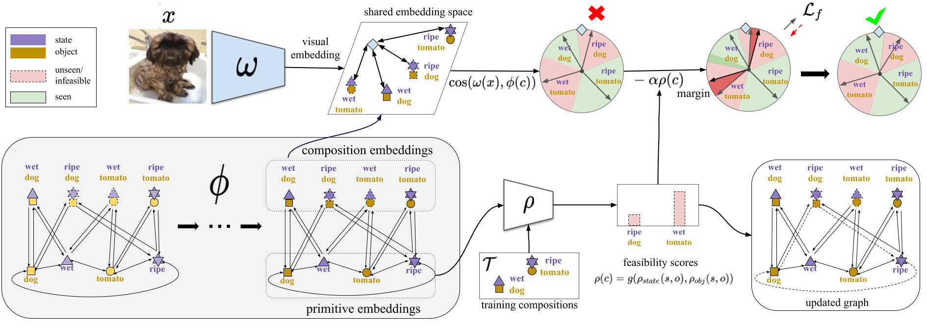
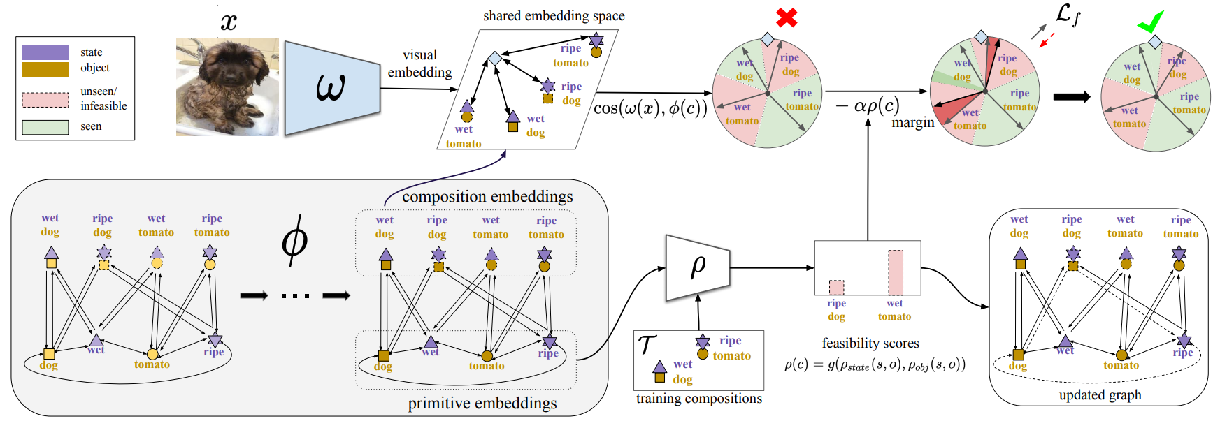 |
|---|
| Our Compositional Cosine Graph Embeddings (Co-CGE) approach for Open World CZSL |
The idea of our approach is simple:
- Project the image into a predefined semantic space.
- Compose object and state descriptions (i.e. word embeddings) into the same semantic space.
- Compute the compatibility (i.e. cosine similarity) between the image and the compositional embeddings to get the final predictions.
Based on the implementations of each component, we name our approach Compositional Cosine Graph-Embeddings (Co-CGE).
Visual projection
The visual projector is a simple convolutional neural network (e.g. ResNet18) with a final multi-layer perception that maps the visual feature to the dimensionality of the shared embedding space.
Graph Embeddings
For the compositional embeddings, we seek a projection function that can extract discriminative embeddings out of each state-object composition. This projection function should be transferrable from seen to unseen compositions. Following our previous work, CGE, we implement this function through a two-layer graph convolutional neural network (GCN). To explain how the graph is built, let's first consider the closed world setting. We take the set of seen and known unseen compositions and we create one node per state, object, and existing composition. We then connect:
- States to the compositions they participate in (and vice-versa)
- Objects to the compositions they participate in (and vice-versa)
- State to objects that participate in the same composition (and vice-versa).
The idea behind the graph is that we can transfer knowledge from seen to unseen compositions through graph connections. As an example, consider a setting where we have as seen compositions: {wet dog, ripe tomato, small cat, wet apple} and as unseen {wet cat}. The representation of the state wet and the object cat are refined within the GCN exploiting the supervision coming from wet dog, wet apple, and small cat. At the same time, those representations are the same that will be used to influence the final embedding of wet cat. This strategy shows amazing results in the closed world. However, how can we connect nodes in the open-world setting where we have no knowledge about test-time unseen compositions? Things get trickier and we need to prune out some connections by exploiting feasibility scores.
Feasibility scores computation
Feasibility scores are values that tell us how likely is to encounter a given composition in the real world. For instance, we should expect wet tomato to have a high feasibility score, while ripe dog to have a pretty low one. We found that it is unclear how to obtain such values from knowledge bases, due to possible missing entries (e.g. dry dog in ConceptNet), and language models, due to misleading co-occurrences (e.g. cored dog due to cored "hot" dog). A possible solution is to go visual, and this is the solution we follow in this work and our previous one, CompCos.
 |
|---|
| The idea behind the computation of the feasibility scores through visual information. |
A dog and a cat are quite similar, right? We can then assume that every state that can be applied to a dog (e.g. dry in the example above) can be applied to cats and vice-versa. Let us suppose we want to compute the feasibility score of wet tomato. We take the graph embedding of tomato and we compute its cosine-similarity with the embeddings of all other objects paired with the state wet in the set of seen compositions (e.g. wet dog, wet apple) since those are the only certain knowledge we can rely on. Our object-based feasibility score is then the maximum of such similarity values (in this case, likely the similarity between tomato and apple). Note that, from the example above, if we check the feasibility score for ripe dog we get a low score, as the cosine similarity between dog and tomato embeddings should be very low to their very different visual appearance. We repeat the same process for the point of view of the states (e.g. for wet tomato we would have checked the similarity between wet and ripe in the above example) and we average these values to get the final feasibility scores. The full process is depicted below.
 |
|---|
| Example of feasibility scores computation (object side) through cosine similarity among embeddings. Yellow denotes seen compositions. |
Exploiting the feasibility scores
Now that we obtained an estimate of the feasibility of each unseen composition, we can use these estimates to enrich our model. In particular, we use the feasibility scores in two ways.
Graph connections.The first is to change the graph connections. In particular, we consider as valid all compositions whose feasibility score is positive. We then consider all valid compositions to build the graph, as previously described but by setting the weight of some of the edges equal to the feasibility scores. In particular, we replace with use the feasibility scores for:
- The connections between states and objects
- The connection from compositions to their primitives (i.e. object and states)
In this way, the objects and states representations are less influenced by less feasible compositions. We found this to be largely beneficial for the final performance of our model. The graph is updated over time as we get improved estimates of state and object embeddings.
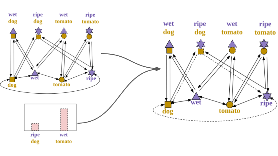 |
|---|
| Graph connections update through the feasibility scores (pink bars). Connections linked to less feasible compositions (ripe dog) are weaker (dashed lines on the right). |
Loss function. We follow CompCos and we train the model using a classification loss where the score of a composition is the cosine similarity between the image embedding and the composition embeddings.
Results
We test our model on various challenging benchmarks, namely:
- MIT-States, containing photos of 245 objects in 115 states;
- UT-Zappos, a dataset of shoes with 12 types and 16 attributes;
- C-GQA, a recently proposed large-scale benchmark with 870 objects in 453 states.
We compare our approach with multiple state-of-the-art methods:
Moreover, we compare our model with our previously proposed compositional graph embedding for the closed world setting (CGE) and our compositional cosine logits approach (CompCos) firstly adopted for the open-world setting.
Overall, the results show that our full method is the best or comparable to the best in all datasets for the closed world:
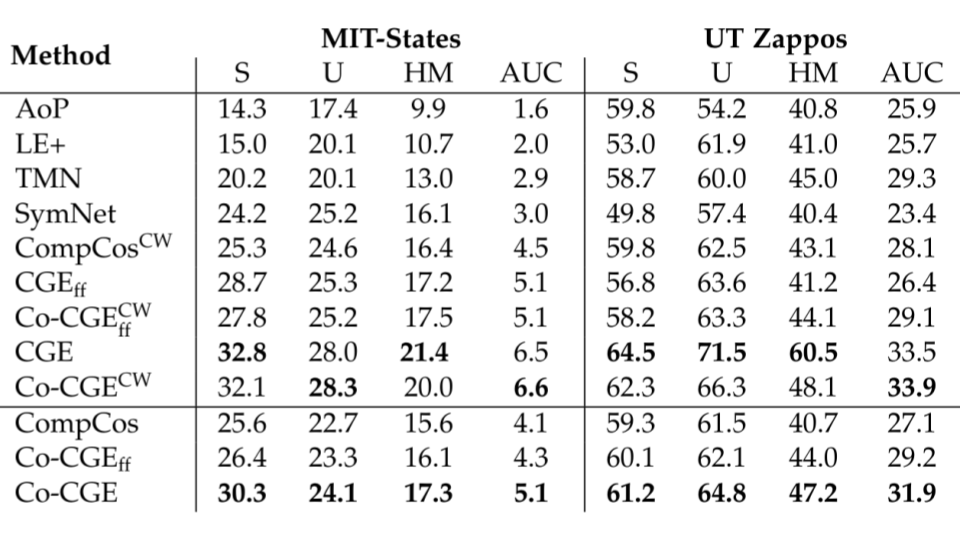 |
|---|
| Results for Closed World CZSL, the superscript CW indicates no use of feasibility scores, the subscript ff indicates no fine-tuning. |
while being superior to all other approaches in the open-world setting:
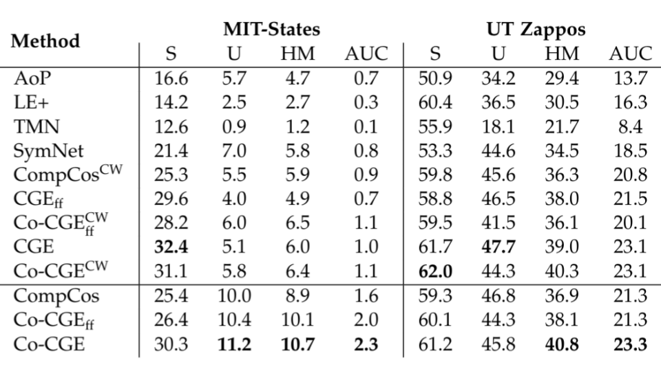 |
|---|
| Results for Open World CZSL, the superscript CW indicates no use of feasibility scores, the subscript ff indicates no fine-tuning. |
It is interesting to highlight how modeling the feasibility of each unseen composition is crucial to achieving reliable predictions. For instance, while our model without feasibility scores (Co-CGE^CW) classifies a wrinkled elephant as a coiled one or a brown bun as a glazed blanket, our full model (Co-CGE) correctly classifies both instances. Of course, our model is still not perfect, but it gives more reasonable predictions when it fails than its closed-world counterpart, as predicting a small snake rather than a rusty one, or a sliced chicken rather than a viscous one (see examples below).
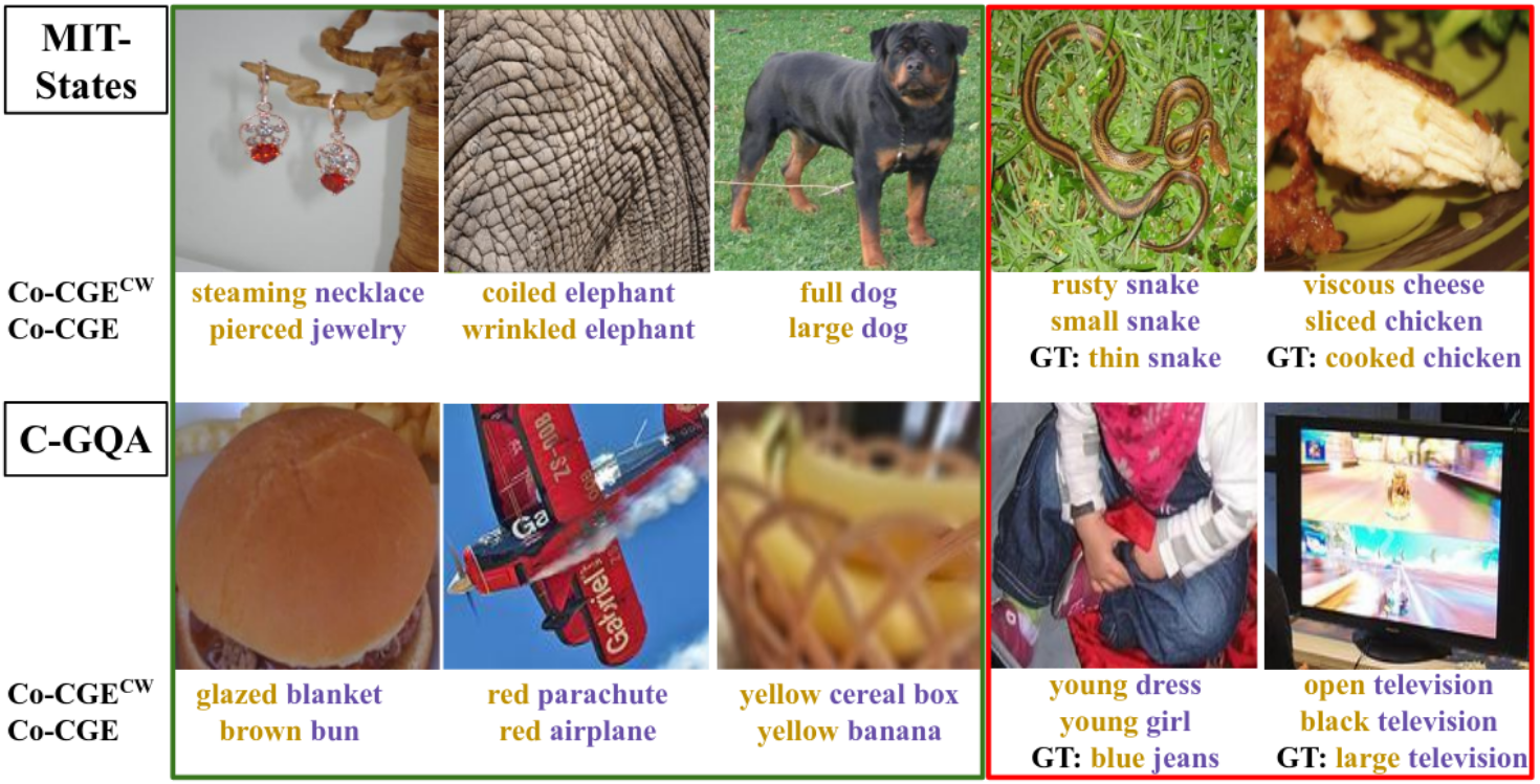 |
|---|
| Qualitative results of our model with (Co-CGE) and without Co-CGE^CW) using feasibility scores for sample images of MIT-States (top) and C-GQA (bottom). |
Conclusions
In this post, we discussed Co-CGE, our recent approach for open-world compositional zero-shot learning. Co-CGE models the relationship between primitives and compositions through a graph convolutional neural network. Co-CGE models the feasibility of a state-object composition by using the visual information available in the training set, incorporating feasibility scores in two ways: as margins for a cross-entropy loss and as weights for the graph connections. The results of Co-CGE on various benchmarks and settings, clearly show the promise of such an approach.
In the future, it would be interesting to explore other ways of computing the feasibility scores (e.g. through external knowledge) and of incorporating them within the model.
You can find more details of this post in our paper and try out some of our CZSL models here.