Long Summary

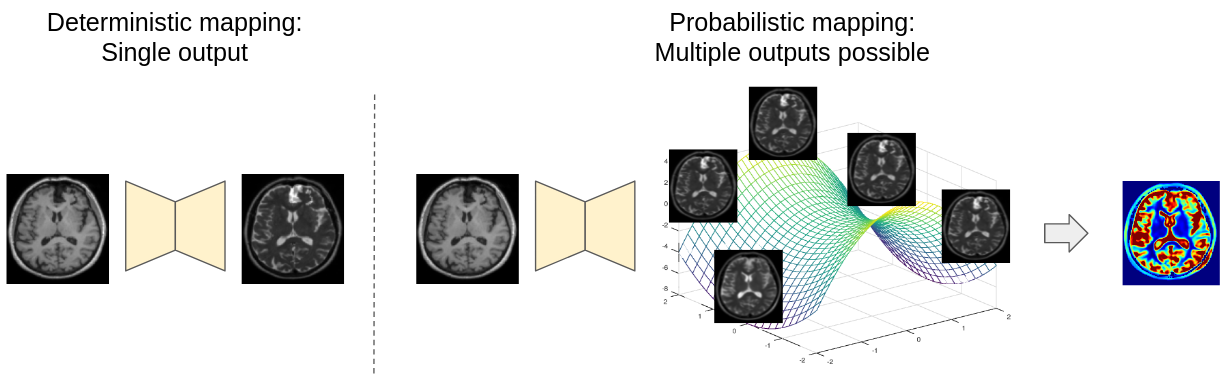
Translating an image from a distribution, i.e. source domain, to an image in another distribution, i.e. target domain, with a distribution shift is an ill-posed problem as a unique deterministic one-to-one mapping may not exist between the two domains. Furthermore, since the correspondence between inter-domain samples may be missing, their joint-distribution needs to be inferred from a set of marginal distributions. However, as infinitely many joint distributions can be decomposed into a fixed set of marginal distributions, the problem is ill-posed in the absence of additional constraints. Image translation approaches often learn a deterministic mapping between the domains where every pixel in the input domain is mapped to a fixed pixel value in the output domain. However, such a deterministic formulation can lead to mode collapse while at the same time not being able to quantify the model predictive uncertainty important for critical applications, e.g., medical image analysis. We propose an unpaired probabilistic image-to-image translation method trained without inter-domain correspondence in an end-to-end manner. The probabilistic nature of this method provides uncertainty estimates for the predictions. Moreover, modelling the residuals between the predictions and the ground-truth with heavy-tailed distributions makes our model robust to outliers and various unseen data.

Notations

Let there be two image domains $A$ and $B$. Let the set of images from domain $A$ and $B$ be defined by (i) $S_{A} := \{a_1, a_2 ... a_n\}$, where $a_i \sim \mathcal{P}_A \forall i$ and (ii) $S_{B} := \{b_1, b_2 ... b_m\}$, where $b_i \sim \mathcal{P}_B \forall i$, respectively. The elements $a_i$ and $b_i$ represent the $i^{th}$ image from domain $A$ and $B$ respectively, and are drawn from an underlying unknown probability distribution $\mathcal{P}_{A}$ and $\mathcal{P}_{B}$ respectively.

Let each image have $K$ pixels, and $u_{ik}$ represent the $k^{th}$ pixel of a particular image $u_i$. We are interested in learning a mapping from domain $A$ to $B$ ($A \rightarrow B$) and $B$ to $A$ ($B \rightarrow A$) in an unpaired manner so that the correspondence between the samples from $\mathcal{P}_A$ and $\mathcal{P}_B$ is not required at the learning stage. In other words, we want to learn the underlying joint distribution $\mathcal{P}_{AB}$ from the given marginal distributions $\mathcal{P}_A$ and $\mathcal{P}_B$. This work utilizes CycleGANs that leverage the cycle consistency to learn mappings from both directions ($A \rightarrow B$ and $B \rightarrow A$).

Cycle Consistency and its interpretation as Maximum Likelihood Estimation (MLE)

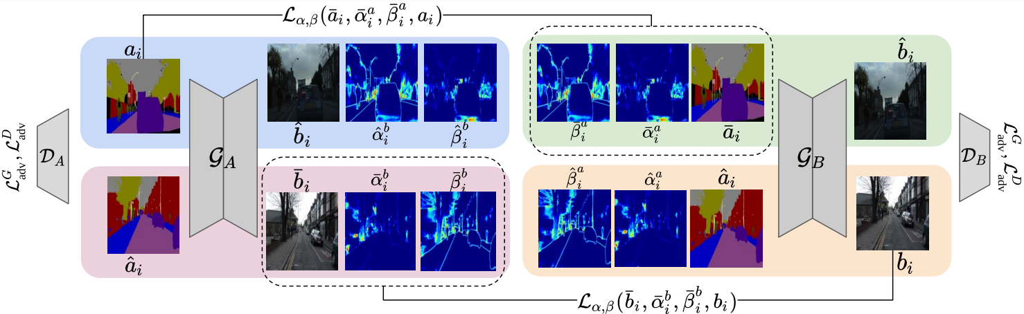
CycleGAN enforces an additional structure on the joint distribution using a set of primary networks (forming a GAN) and a set of auxiliary networks. The primary networks are represented by $\{\mathcal{G}_A(\cdot; \theta^\mathcal{G}_A), \mathcal{D}_A(\cdot; \theta^\mathcal{D}_A)\}$, where $\mathcal{G}_A$ represents a generator and $\mathcal{D}_A$ represents a discriminator. The auxiliary networks are represented by $\{\mathcal{G}_B(\cdot; \theta^\mathcal{G}_B), \mathcal{D}_B(\cdot; \theta^\mathcal{D}_B)\}$. While the primary networks learn the mapping $A \rightarrow B$, the auxiliary networks learn $B \rightarrow A$. Let the output of the generator $\mathcal{G}_A$ translating samples from domain $A$ (say $a_i$) to domain $B$ be called $\hat{b}_i$. Similarly, for the generator $\mathcal{G}_B$ translating samples from domain $B$ (say $b_i$) to domain $A$ be called $\hat{a}_i$, i.e., $\hat{b}_i = \mathcal{G}_A(a_i; \theta^{\mathcal{G}}_A) \text{ and } \hat{a}_i = \mathcal{G}_B(b_i; \theta^{\mathcal{G}}_B)$. To simplify the notation, we will omit writing parameters of the networks in the equation. The cycle consistency constraint re-translates the above predictions ($\hat{b}_i, \hat{a}_i$) to get back the reconstruction in the original domain ($\bar{a}_i$,$\bar{b}_i$), where, $\bar{a}_i = \mathcal{G}_B(\hat{b}_i) \text{ and } \bar{b}_i = \mathcal{G}_A(\hat{a}_i),$ and attempts to make reconstructed images ($\bar{a}_i, \bar{b}_i$) similar to original input ($a_i, b_i$) by penalizing the residuals with $\mathcal{L}_1$ norm between the reconstructions and the original input images, giving the cycle consistency,

The underlying assumption when penalizing with the $\mathcal{L}_1$ norm is that the residual at \textit{every pixel} between the reconstruction and the input follow \textit{zero-mean and fixed-variance Laplace} distribution, i.e., $\bar{a}_{ij} = a_{ij} + \epsilon^a_{ij}$ and $\bar{b}_{ij} = b_{ij} + \epsilon^b_{ij}$ with,

where $\sigma^2$ represents the fixed-variance of the distribution, $a_{ij}$ represents the $j^{th}$ pixel in image $a_i$, and $\epsilon^{a}_{ij}$ represents the noise in the $j^{th}$ pixel for the estimated image $\bar{a}_{ij}$. This assumption on the residuals between the reconstruction and the input enforces the likelihood (i.e., $\mathscr{L}(\Theta | \mathcal{X}) = \mathcal{P}(\mathcal{X}|\Theta)$, where $\Theta := \theta^{\mathcal{G}}_A \cup \theta^{\mathcal{G}}_B \cup \theta^{\mathcal{D}}_A \cup \theta^{\mathcal{D}}_B$ and $\mathcal{X}:= S_A \cup S_B$) to follow a factored Laplace distribution:

where minimizing the negative-log-likelihood yields $\mathcal{L}_{\text{cyc}}$ with the following limitations. The residuals in the presence of outliers may not follow the Laplace distribution but instead a heavy-tailed distribution, whereas the i.i.d assumption leads to fixed variance distributions for the residuals that do not allow modelling of heteroscedasticity to aid in uncertainty estimation.

Building Uncertainty-aware Cycle Consistency

We propose to alleviate the mentioned issues by modelling the underlying per-pixel residual distribution as independent but non-identically distributed zero-mean generalized Gaussian distribution} (GGD), i.e., with no fixed shape ($\beta > 0$) and scale ($\alpha > 0$) parameters. Instead, all the shape and scale parameters of the distributions are predicted from the networks and formulated as follows:

For each $\epsilon_{ij}$, the parameters of the distribution $\{\bar{\alpha}_{ij}, \bar{\beta}_{ij}\}$ may not be the same as parameters for other $\epsilon_{ik}$s; therefore, they are non-identically distributed allowing modelling with heavier tail distributions. The likelihood for our proposed model is,

where ($\bar{\beta}^a_{ij}$) represents the $j^{th}$ pixel of domain $A$'s shape parameter $\beta^a_i$ (similarly for others). $\mathscr{G}(\bar{\beta}^u_{ij},\bar{\alpha}^u_{ij},\bar{u}_{ij},u_{ij})$ is the pixel-likelihood at $j^{th}$ pixel of image $u_i$ (that can represent images of both domain $A$ and $B$) formulated as, $\mathscr{G}(\bar{\beta}^u_{ij},\bar{\alpha}^u_{ij},\bar{u}_{ij},u_{ij}) = GGD(u_{ij}; \bar{u}_{ij}, \bar{\alpha}^u_{ij}, \bar{\beta}^u_{ij}).$

The negative-log-likelihood is given by,

minimizing the negative-log-likelihood yields a new cycle consistency loss, which we call as the uncertainty-aware generalized adaptive cycle consistency loss $\mathcal{L}_{\text{ucyc}}$, given $\mathscr{A}=\{\bar{a}_i, \bar{\alpha}^{a}_i, \bar{\beta}^{a}_i, a_i\}$ and $\mathscr{B}=\{\bar{b}_i, \bar{\alpha}^{b}_i, \bar{\beta}^{b}_i, b_i\}$,

where $\mathcal{L}_{\alpha\beta}(\mathscr{A}) = \mathcal{L}_{\alpha\beta}(\bar{a}_i, \bar{\alpha}^{a}_i, \bar{\beta}^{a}_i, a_i)$ is the new objective function corresponding to domain $A$,

where $(\bar{a}_i, \bar{b}_i)$ are the reconstructions for $(a_i,b_i)$ and $(\bar{\alpha}^{a}_i, \bar{\beta}^{a}_i), (\bar{\alpha}^{b}_i, \bar{\beta}^{b}_i)$ are scale and shape parameters for the reconstruction $(\bar{a}_i, \bar{b}_i)$, respectively. The $\mathcal{L}_1$ norm-based cycle consistency $\mathcal{L}_{\text{cyc}}$ is a special case of $\mathcal{L}_{\text{ucyc}}$ with $(\bar{\alpha}^{a}_{ij}, \bar{\beta}^{a}_{ij}, \bar{\alpha}^{b}_{ij}, \bar{\beta}^{b}_{ij}) = (1,1,1,1) \forall i,j$. To utilize $\mathcal{L}_{\text{ucyc}}$, one must have the $\alpha$ maps and the $\beta$ maps for the reconstructions of the inputs. To obtain the reconstructed image, $\alpha$ (scale map), and $\beta$ (shape map), we modify the head of the generators (the last few convolutional layers) and split them into three heads, connected to a common backbone.

Once we train the model, for every input image, the model will provide the scale ($\alpha$) and the shape ($\beta$) maps that can be used to obtain the aleatoric uncertainty given by,

To see the resulting uncertainty maps along with our perturbation analysis of the trained model please check Section 4 of the paper.